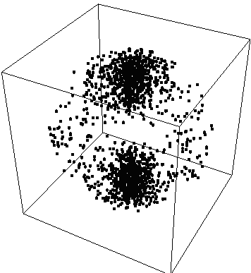
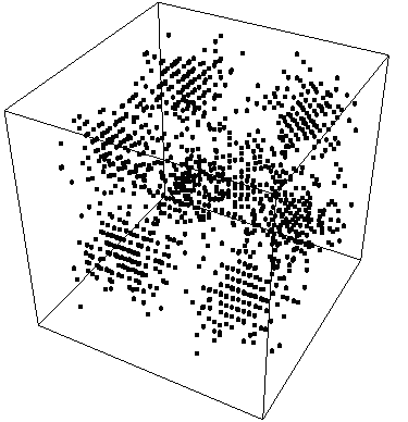
 {fig 1}
An offline version of this page, and the probability plotter can be obtained here
The purpose of this web page is to demonstrate the use of
the probability density plotter using some basic wavefunctions.
In the images,
the density of points is proportional to the probability density/unit volume.
We start with a simple example, the particle in a box of length L=2 Pi
Psi[x,y,z]=A*Sin[x]*Sin[y]*Sin[z]
With V=0 Abs[x] <=L, that is the potential is zero inside the box
and V=Infinite Abs[x]>L
So Psi*Psi=A^2*Sin[x^2]*Sin[y]^2*Sin[z]^2
In order to achieve the proper probability density distribution
we must take Psi*Psi, Integrate it over the limits 0<x<L, 0<y<L,
0<z<L So…
Integrate[Sin[x]^2*Sin[y]^2*Sin[z]^2,{x,0,2 Pi},{y,0,2 Pi},{z,0,2
Pi}]
=A^2 Pi^3
Therefore Psi=A*Pi^(-3/2)*(Sin[x]*Sin[y]*Sin[z])
To produce a clear image, we will choose A=1/Pi^(-3/2)
Psi=Sin[x]*Sin[y]*Sin[z]
ProbabilityPlot[Psi^2,{x,0,2 Pi,.3},{y,0,2 Pi,.3},{z,0, 2 Pi,.3}] produces:
 {fig 1}
Choosing a single slice of this and overlaying an x-y plot of the probability density in the plane z=Pi/2
ProbabilityPlot[Psi^2,{x,0,2 Pi,.3},{y,0,2 Pi,.3},{z,Pi/2,Pi/2}]
produces:
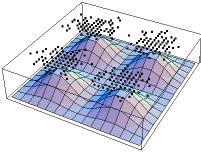
From this, we can see that the highest probability areas contain the most points whereas the lowest contain the least, as expected
{fig2}
For our next example, we will do a calibration plot, in spherical coordinates of the probability density function Psi*Psi=r^2
So,
ProbabilityPlotSpherical[r^2,{r,0,1,.1},{theta,0, Pi,.1},{phi,.3}]
produces:
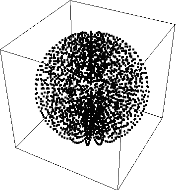 {fig3}
Unfortunately, this doesn't tell us much, so we'll take a slice of it…
ProbabilityPlotSpherical[r^2,{r,0,1,.1},{theta,0,Pi,.1},{phi,0,0}]
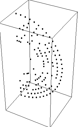 As expected, the density is low in the center and high
at the edges
{fig4}
Now for the last demonstrations we take the Psi310 and Psi320 states of the hydrogen atom. The wavefunctions of the 310 state take the form of:
Psi=r*(1-r)*Exp[-r]*Cos[theta].
Here we have left off various constant multiples, such as the Bohr radius and the atomic number, since we are just interested in the form of the distribution, not numerical quantities.
We want to scale this so that everything interesting
happens between r=0 and r=1 hence speeding up the plot…therefore we first plot
the square of the radial part of Psi (since in the end it is Psi^2 that is plotted)
This produces:
{fig5}
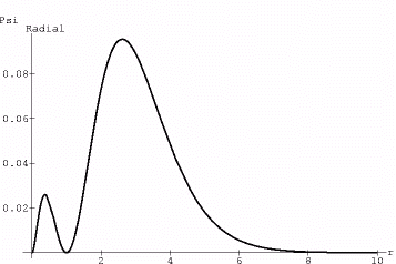 By making the replacement r=k*r where k is the scaling factor we get
the dsired result of making the interesting parts of fig5 fit between 0 and
1, likewise, we multiply the entire radial portion by another scaling factor
to ensure our probabilities are reasonably distributed.
Psiradial=A*f[k*r], where f is the wavefunction
We choose k=10 and A=10 for proper scaling. We then proceed to plot Psi*Psi
and get: 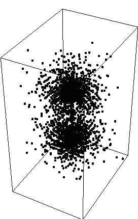 {fig6}
and {fig6a}
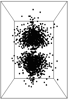
The wavefunctions of the 320 state take the form of Psi=r^2*Exp[-r]*(3*Cos[theta]^2-1)
So, again, we start by scaling the radial portion of the wavefunction,
Plot[r^2*Exp[-2*r],{r,0,10}]
{fig7}
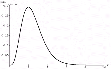
setting k=10 provides the proper scaling…
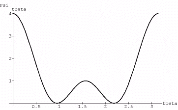
Now the theta portion plots like:
{fig8}
Multiplying this by 1/4 and Psiradialand plotting Psi*Psi we get:
{fig9}
